How to add error bars in Excel: A quick tutorial
What are error bars and what do they indicate in Excel? They are unique tools used in the graphical representation of data. Some people still do not know how to add error bars in Excel. Well, we have several techniques that will guide you to get this done.
Source: UGC
Perhaps you are wondering, "What do error bars show in a chart or graph?" They are used to display margins of mistakes, including how far the actual figures might be compared to the reported values in the presentation. Besides, they provide a clear view of data, and one can quickly tell the margins. Another advantage is that they are available in both Windows and Mac Excels.
How to add error bars in Excel
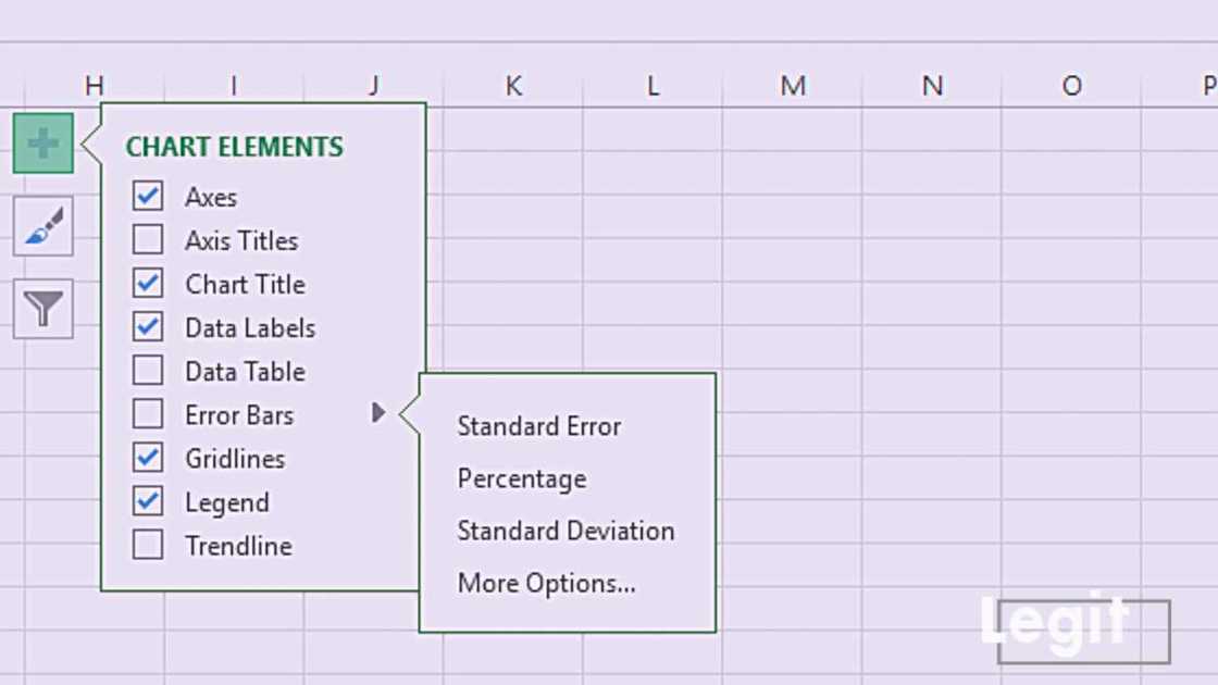
You can insert these tools in numerous presentations including in a 2-D bar, column, XY (scatter) plot, bubble chart, line, and area graph. The Excel tool has three different classifications.
- Standard Error – It is the first option appearing on the drop-down. It shows the standard error for all values in the data set.
- Percentage – It determines the amount of error and percentage range for each value, although you can also set your preferred rate.
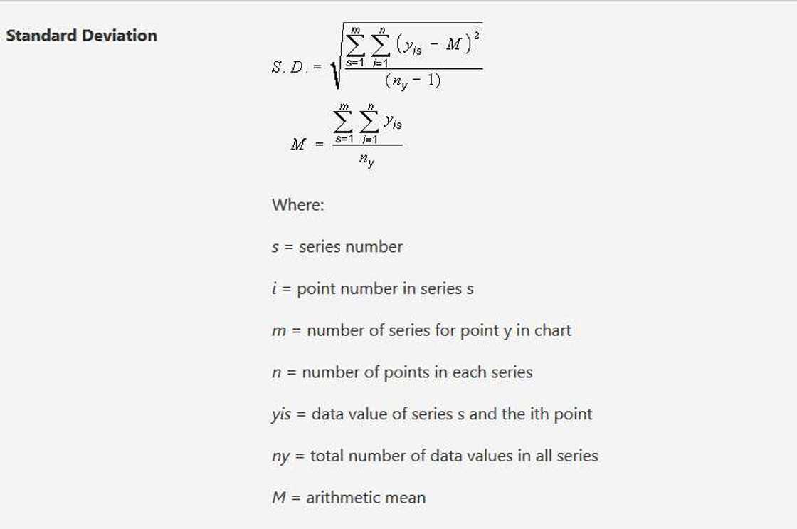
- Standard Deviation – It displays a standard deviation for the data, including how close it is to the average.
Source: Original
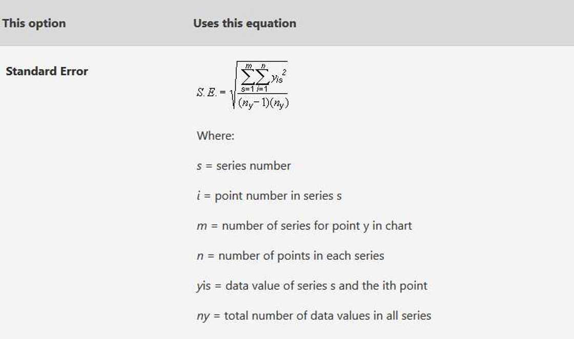
Microsoft Excel has a unique formula for calculating error bars, which varies according to the type.
For percentage, they display a value of 5% in Excel; however, for Standard type, the following formula is used to determine their amounts.
Source: UGC
Standard Deviation uses the formula below.
Source: UGC
Inserting error bars in Excel 2013, 2016, and 2019
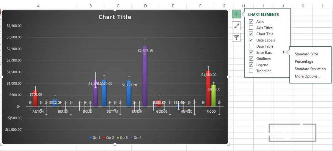
Generally, the procedure used to add error bars Excel 2016 and 2019 is similar to that of 2013 version. You need to perform the following steps:
- Click on your chart.
- Proceed to chart elements by clicking the thick plus (+) sign.
- Go to the Error Bars element and click the arrow next to it.
- Select your preferred type in the drop-down.
Source: Original
- The changes come into effect immediately in the chart.
- If you choose More Options, you can easily make modifications according to your preference.
READ ALSO: How to split cells in Excel: An easy tutorial
Adding error bars in Excel 2010 and 2007
Note that the path followed when working with Excel 2010 and 2007 is different from that of the subsequent versions. This, however, does not mean that we can ignore the two older versions since there are people who still use them. Their users would also love to unlock the secret of using the tool in their respective Microsoft versions. We, therefore, take a look at the procedure:
- Click on your chart to display Chart Tools on the header.
- Under the Chart Tools, select the Layout tab.
- Navigate through and choose an option from the list in the drop-down.
- To remove everything, click the None option. You can also customize by selecting more options at the bottom of the drop-down.
Customization error bars in Excel
In case you are not impressed with the standard options provided, the best thing is to modify the existing settings by making adjustments that suit your needs.
- Navigate through the initial steps as described in the previous processes and select the More Options element.

Source: Original
- A new formatting menu will appear on the right side of the Windows.
- Scroll down the menu and select Custom located at the bottom.
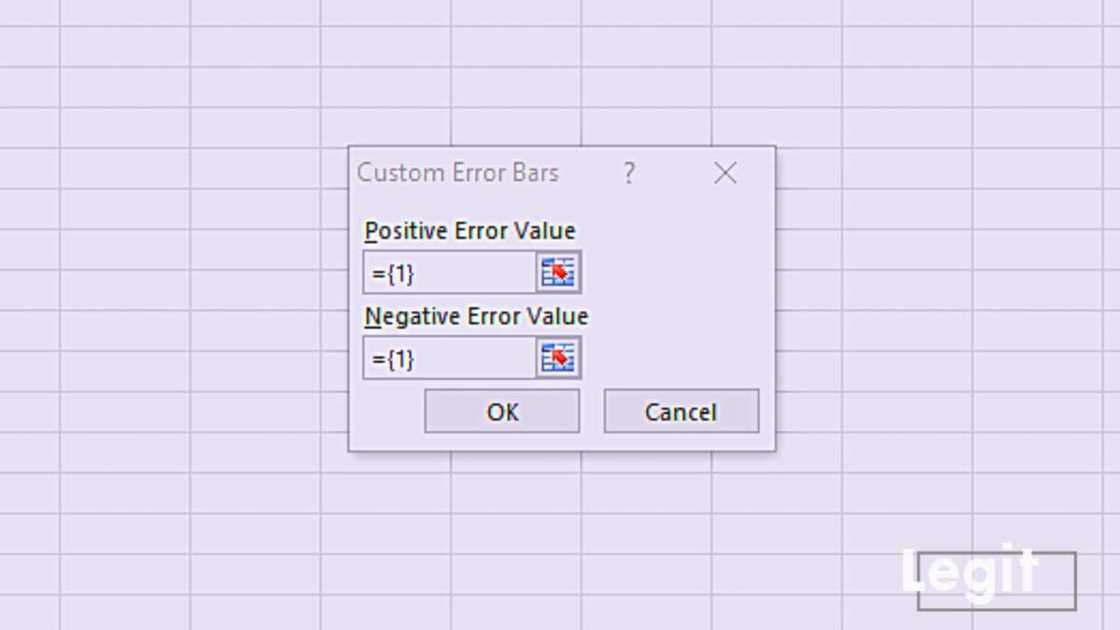
- Next, click the Specific Value option. A small log box will pop-up on your window with two slots to fill.
Source: Original
- Add your preferred values in the positive or negative value boxes.
- Click OK to display the changes in the chart.
Horizontal error bars
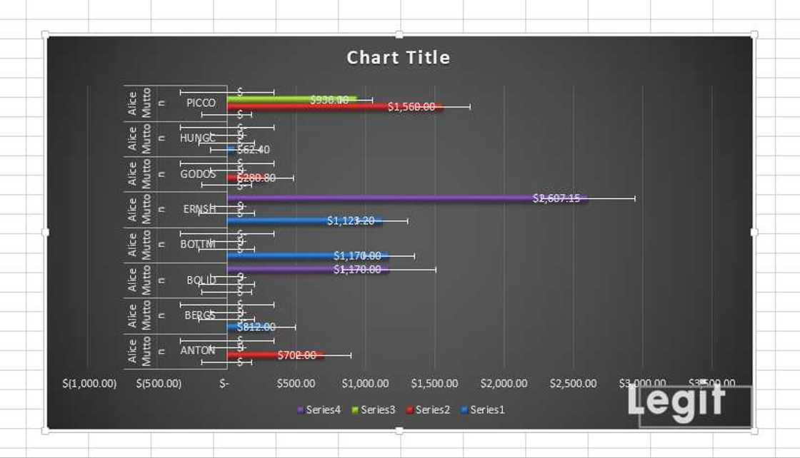
Is it possible to add horizontal error bars to Excel presentations? When dealing with charts, you do not need to worry much since they are the only type found in bar charts. Once you add them, they display immediately. A similar case applies to the vertical type, which also appears by default in column charts once added.
Source: Original
The problem comes when working with a bubble or a scatter graph. Here, you must remove the vertical and add the horizontal ones, but how do you accomplish this?
- Use the steps in previous procedures to add vertical error bars to your chart.
- To remove them, right-click any of them available in the chart and choose Delete option from the drop-down.
- Open the Format Error Bars menu and customize the horizontal type.
How to add error bars in Excel for Mac
Apart from Windows, you can also add Excel error bars for Mac, but with a different yet straightforward path and process:
- Click on your data or chart, then proceed to Chart Design tab on the header.
- Go to the Add Chart Element, select to bring options in the drop-down.
- Continue navigating through the same path as in Windows and press OK after completing the procedure.
- The changes will be effected immediately on the data.
If you want to customize your values, the same process applies as in Windows:
- Instead of choosing your preferred type as above, explore more options on the bottom of the drop-down.
- Proceed to the new window and move down to the Error Amount section in the new window, click Custom and then the Specify Value option.
- Fill the two parts in the small window with your positive and negative values.
- Type your preferred figures and then click OK to make changes in the chart.
You are now familiar with how to add error bars in Excel both for Windows and Mac operating systems. You can now easily add the tool in your chart or graphical presentation. Reach out to friends and colleagues and help them when they stranded on what to do. Maybe one day the skill may earn you some cash somewhere.
READ ALSO: How to find and remove duplicates Excel: Tutorial
Source: Legit.ng


